SpectroPipeR - step 5 - reporting • SpectroPipeR

If you want to have a closer look at the images and plots just do a “right-click” on the image and select “open in new tab”

The output folders contained figures that were always exported in two file formats: vector PDF and raster PNG.

Recommendations for MacOS Users

For MacOS users, it is recommended to use the PDF files, for example in Keynote, to achieve better quality.

Recommendations for Windows Users

For Windows users, it is recommended to use the PNG files, as applications like Microsoft PowerPoint can sometimes have issues when working with vector graphics.

SpectroPipeR reporting

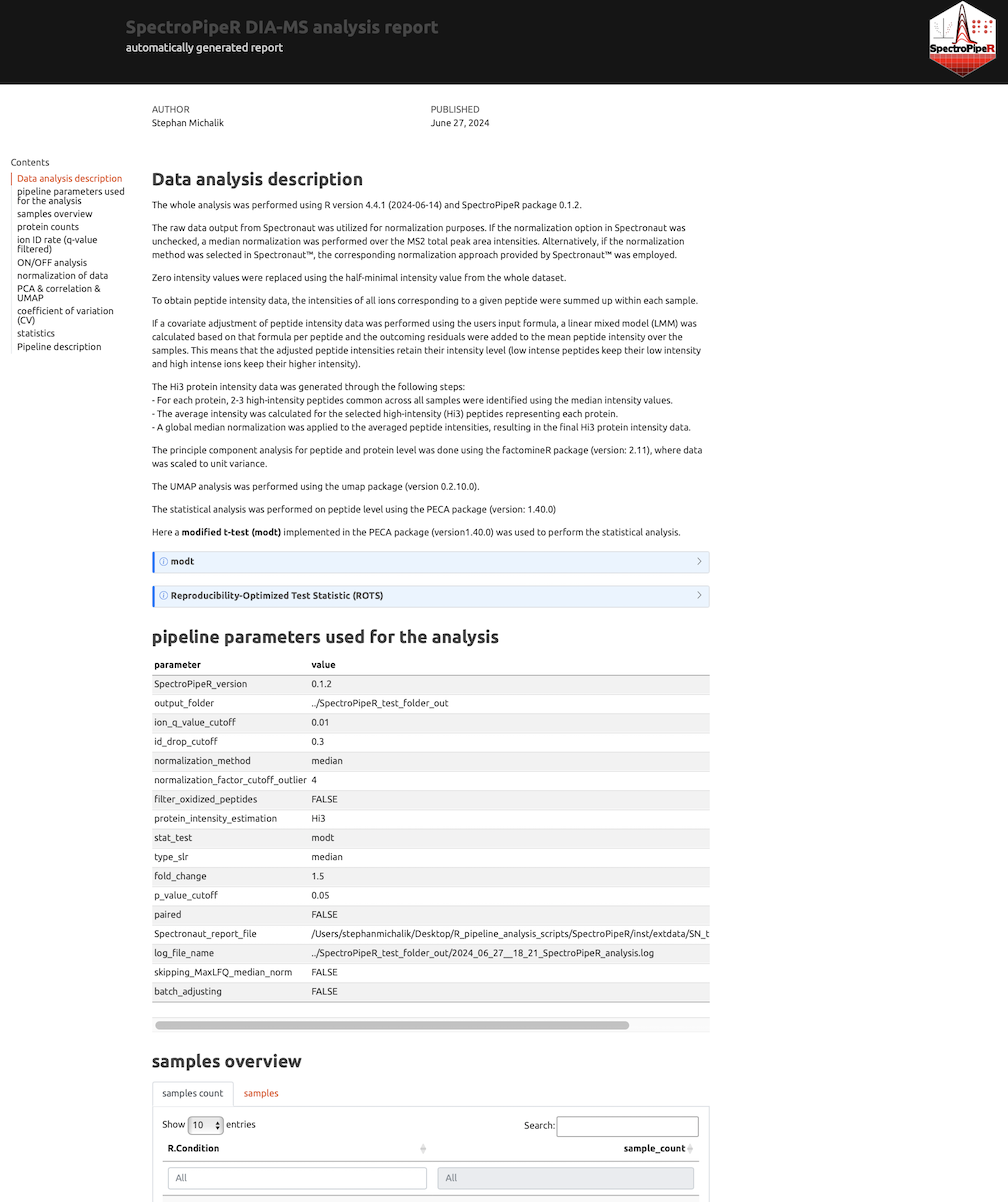
The reporting module takes the inputs from:

step 1 - read Spectronaut data
step 2 - normalization and quantification
step 5 - statistics (optional)

to render an interactive standalone HTML report. The rendering is performed with Quarto CLI. So Quarto CLI is required. If you did not already install the Quarto CLI you should install the Quarto CLI using Quarto get started installation.

SpectroPipeR functions executed before

# parameter list
params <- list(output_folder = "../SpectroPipeR_test_folder")

# example input file, bundled with SpectroPipeR package
example_file_path <- system.file("extdata", "SN_test_HYE_mix_file.tsv", package="SpectroPipeR")

# step 1: load Spectronaut data module
SpectroPipeR_data <- read_spectronaut_module(file = example_file_path,
                                      parameter = params,
                                      print.plot = FALSE)

# step 2: normalize & quantification module
SpectroPipeR_data_quant <- norm_quant_module(SpectroPipeR_data = SpectroPipeR_data,print.plot = FALSE)

# step 3: MVA module
MVA_module(SpectroPipeR_data_quant = SpectroPipeR_data_quant)

# step 4: statistics module
SpectroPipeR_data_stats <- statistics_module(SpectroPipeR_data_quant = SpectroPipeR_data_quant,
                                       condition_comparisons = cbind(c("B_manual","A_manual")))

Report generation

# step 5: report module
SpectroPipeR_report_module(SpectroPipeR_data = SpectroPipeR_data,
                     SpectroPipeR_data_quant = SpectroPipeR_data_quant,
                     SpectroPipeR_data_stats = SpectroPipeR_data_stats)

# #*****************************************
# # REPORT MODULE
# #*****************************************
# 
# generating methods part ...
# render HTML report ... this might take a while 
# 
# processing file: DIA_MS_analysis_report_Master.qmd
#   |...............                                    |  30%                   # A tibble: 1 × 1
#   value
#   <chr>
# 1 0.01 
#                                           
# output file: DIA_MS_analysis_report_Master.knit.md
# 
# pandoc --output SpectroPipeR_report.html
#   to: html
#   standalone: true
#   self-contained: true
#   section-divs: true
#   html-math-method: katex
#   wrap: none
#   default-image-extension: png
#   css:
#     - styles.css
#   toc: true
#   toc-depth: 3
#   
# metadata
#   document-css: false
#   link-citations: true
#   date-format: long
#   lang: en
#   title: SpectroPipeR DIA-MS analysis report
#   author: Stephan Michalik
#   date: '`r format(Sys.Date(), "%B %d, %Y")`'
#   title-block-banner: '#151515'
#   subtitle: automatically generated report
#   page-layout: full
#   toc-title: Contents
#   theme: united
#   highlight: tango
#   df_print: paged
#   toc-location: left
#   anchor-sections: true
#   smooth-scroll: true
#   
# Output created: SpectroPipeR_report.html
# 
# render HTML report ... DONE!

SpectroPipeR_report_module() output

SpectroPipeR_report_module() - screenshot of html output report

SpectroPipeR example report

After the function was executed the SpectroPipeR_report.html file was generated inside the output folder.